 octopusgames
Fieldwork · Visual Localization Research Sandbox
This version preserves the Fieldwork navigation view and adds a reproducible experimental workbench. It is a small, transparent synthetic localization system, not an implementation of a production visual navigation stack.
- Measured experiments and interpretation
- Raw benchmark JSON
- Every observation, learning pass and ablation in CSV
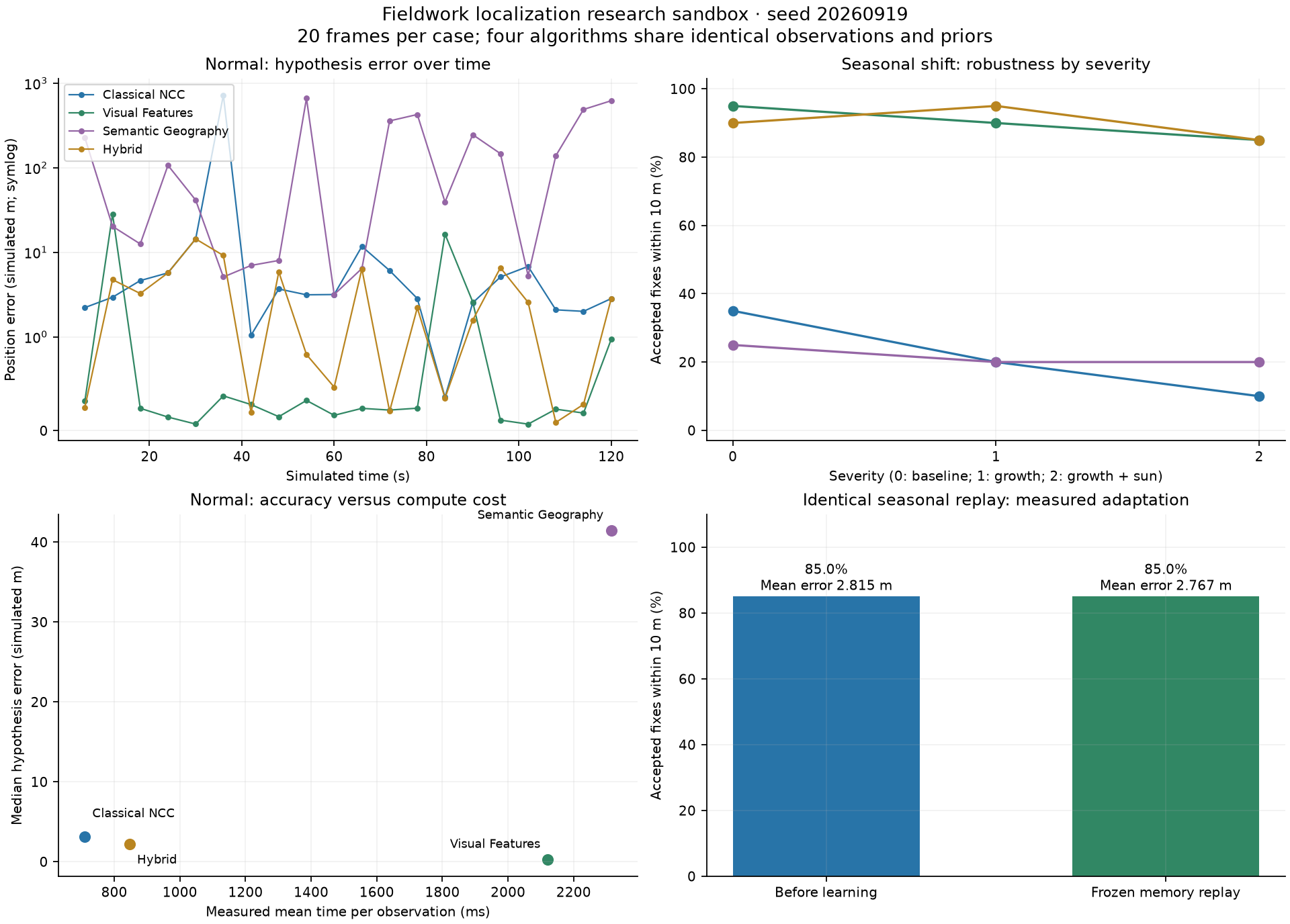
- Four experiment figures, PDF
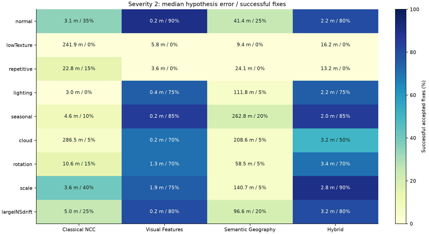
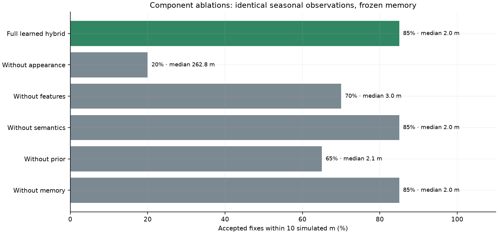
- Algorithm × scenario matrix, component ablations
Architecture and information boundaries
flowchart TD
 W[Immutable latent world: infrastructure, parcels, trees, elevation] --> R[Historical acquisition: Day 0]
 W --> L[Independent live acquisition: Day 30 or seasonal Day 120]
 R --> I[Reference image index and image-derived geography]
 L --> O[EO projection, GSD, yaw, blur, clouds and noise]
 O --> Q[Observed descriptors, corners, components and relations]
 I --> G[Global retrieval: Top 3]
 Q --> G
 P[Navigation prediction and uncertainty] --> G
 G --> M[Method-specific matching and local pose search]
 M --> V[Evidence, ambiguity and geometric verification]
 V --> S[Accepted pose / rejected observation]
 S --> F[Illustrative navigation correction state]
 S --> T[High-confidence + geometry + innovation gate]
 T --> A[Stored observed appearance and descriptors]
 A --> G
 W -. evaluator truth only .-> E[Benchmark position / heading / scale error]
 S --> E
terrain.js owns the deterministic immutable world and acquisition renderers. Reference and live acquisitions are separate renders of that world, with different growth, sun and sensor response. sensor.js projects either acquisition into a 192 × 192 EO observation, with a nominal 96 simulated metre footprint. Rotation, scale and the map footprint share the projection geometry. A live observation never samples the historical raster.
geography.js constructs the latent scene graph and separately extracts image evidence. localization.js accepts only a captured observation, nominal camera pose and navigation prior. It has no access to the evaluator's true pose or disturbance labels. memory.js stores estimator-verified observations. model.js connects pose decisions to the live navigation state. benchmark.js alone owns ground truth for generating observations and measuring errors. benchmark-worker.js runs browser experiments off the UI thread; research-ui.js only presents returned measurements.
Geographic representation
The latent graph contains road centerlines, an intersection, bridge/crossing, river and curvature extrema, parcel and woodland boundaries, individual tree entities, building footprints/corners/cluster, elevation regions and configurations. Each entity has a type, position, geometry, orientation, scale, local/semantic descriptors and a heuristic distinctiveness. Parcel cells follow the renderer's weighted nearest-field metric; woodland outlines use its irregular boundary function.
Immutable graph entities have an external observation-history map keyed by feature ID. Verified image features are projected using the estimated pose and associated to compatible nearby graph entities. These are explicitly estimated associations, not ground-truth labels. This audit history is never fed into the matcher.
Image geography is an intentionally modest, transparent extractor. It measures material-color components, contours, pixel PCA orientation, texture direction and corners. It creates conservative road, water, vegetation, field and roof-like hypotheses. It can confuse bare soil with a roof or a grey roof with road material. It does not declare an unseen bridge merely because water is nearby.
Structural comparison uses one-to-one same-type component correspondence, normalized pair distances, coherent relative bearings and endpoint-bound relation checks. Visible relations include road/water adjacency, nearby buildings, building/road layout and forest/field adjacency. The inspector reports these measured hypotheses and whether the corresponding candidate supports them. It does not present latent world labels as detected semantics.
Localization algorithms
A cached global lattice of historical reference observations supports retrieval. The normal 1000 × 700 world uses 32 metre lattice spacing and 532 indexed frames. The full measured retrieval surface is displayed in the heatmap. The top three regions undergo local translation, yaw and GSD searches. Coarse candidates can still miss the correct basin; this is a real source of failure.
| Method | Pose and candidate evidence | Verification |
|---|---|---|
| Classical NCC | Normalized luminance correlation on acquired pixels | Measured peak strength and separation |
| Visual Features | Detected corners, local patch descriptors and translation-consistent correspondences | Sufficient inliers and correspondence consistency |
| Semantic Geography | Image-extracted components and their spatial relationships | Measured structural agreement and feature support |
| Hybrid | Appearance, corner evidence, geography and navigation prior | Verification from the enabled evidence channels |
NCC and feature modes share an appearance-based global retrieval front end; semantic retrieval uses extracted structure. A navigation prior can propose an additional historical observation and provide a small retrieval tie-break. Pure methods do not use a hybrid prior weight in final scoring. The prior ablation also removes the prior retrieval proposal and tie-break, so this dependence is measurable.
Heading is derived from the selected image rotation; scale is estimated from the searched image footprint. The yaw and GSD search ranges are deliberately bounded around nominal telemetry. Corner matching is a small patch-descriptor / translation-consensus implementation, not SIFT, SuperPoint, or full projective RANSAC. The terrain camera is nadir and planar; there is no perspective/occlusion-aware 3D bundle adjustment.
Local search is implemented differently across methods: Hybrid uses cheap NCC to propose a local pose before its combined certificate, whereas Feature/Semantic evaluate their structural evidence during pose search. Shared diagnostic measurements are retained for the inspector even when their scoring contribution is disabled. Ablations therefore remove evidence paths, not necessarily every diagnostic CPU cost. Timing describes these particular implementations, not intrinsic algorithm-family complexity.
Confidence is a deterministic heuristic derived from active evidence, candidate ambiguity and measured distinctiveness. It is not a learned or calibrated posterior probability. The benchmark reports empirical calibration separately. There are no random confidence values or algorithm-specific performance presets.
Learning and protection against self-reinforcement
The memory admission gate requires an accepted result, confidence at least 0.55, verified geometry and innovation within two prior standard deviations. The score is heuristic: this threshold is an engineering setting, not a 55% probability statement. Failed admission increments a rejection counter. It stores the acquired appearance, descriptors/geographic hypotheses, estimated pose and reliability, never a true location label.
A learned observation can add a global retrieval proposal. Current adaptation updates the bank of observed appearances/descriptors; it does not re-train a neural network or rewrite the immutable world geometry. Immutable-reference evidence remains authoritative for ranking and verification; learned evidence cannot certify its own acceptance. The same gate is applied on every run. Memory size is bounded. The inspector and learning controls expose admission and stored-record counts; live “gain” is not replaced by an average confidence.
The explicit adaptation experiment records the seasonal sequence once. Pass 1 measures hybrid with memory unavailable to retrieval while storing only verified observations after each decision. Pass 2 replays the exact same images and priors with frozen memory. No new records enter memory during Pass 2. The measured gain is the difference in successful fixes and errors. This is a test of repeated-condition adaptation, not a claim of generalization to held-out imagery.
The training trace also audits admitted observations against evaluator-only truth and reports correct/wrong admissions. These audit labels never enter the memory gate. The poison challenge tests an apparently confident but estimator-inconsistent / geometrically invalid candidate. A rejected update must leave memory empty. This shows the implemented guard behavior; it does not prove that every confident false association is impossible.
Experimental protocol
The default experiment uses seed 20260919, a closed 120 second route, and twenty captured observations at six second intervals. Four algorithms receive exactly the same image objects and numeric priors for a recorded frame. Nine scenarios are evaluated: normal, low texture, repetitive fields, lighting, seasonal shift, clouds, rotation, scale variation and large INS drift. Three severity settings are recorded. Large-INS perturbation bounds are 50, 125 and 250 simulated metres, beyond the nominal image footprint at the stronger settings. Low-texture and repetitive scenes are categorical fixed landscapes; their pixels do not become more degraded with the severity label, while the seeded prior perturbation changes. Actual numeric conditions, frame hashes and source hashes accompany the JSON.
The seed controls repeatable prior perturbations. Terrain and sensor noise use deterministic coordinate/time functions. A changed seed therefore changes the prior sequence, rather than creating an independent geography. Conclusions apply to this synthetic world and route. No randomized multi-map confidence intervals are implied.
The matrix evaluates memory-free methods. The learning experiment evaluates fixed seasonal observations before and after admission into memory. Every ablation removes one enabled component from the same hybrid path and replays the seasonal sequence with the same frozen memory; removing memory supplies no records. The full learned hybrid result is its comparison baseline. Removing appearance also removes appearance-based memory/retrieval proposals, an explicitly coupled intervention.
| Metric | Exact meaning |
|---|---|
| Hypothesis error | Euclidean estimated-vs-true x/y error, including rejected answers |
| Median / p95 | Empirical nearest-rank quantiles of all hypothesis errors; accepted-only values also exported |
| Successful localization | Accepted and within the configured 10 simulated metre tolerance |
| False match | Accepted outside tolerance; UI denominator is all observations |
| Rejected rate | Rejected observations / all observations |
| Recovery | Time from a failure episode to the next successful accepted fix; unrecovered episodes remain right-censored |
| Domain-shift robustness | Measured success/error at each severity, not an invented robustness index |
| Compute cost | Measured elapsed localization time per observation, excluding index construction; environment dependent |
| Search count | Actual detailed pose evaluations; index size/build time reported separately by engine |
| Calibration | Five empirical bins of heuristic confidence against successful accepted fixes; ECE is descriptive |
| Adaptation | Paired frozen-memory replay; improvement, no change or deterioration are all reported |
Reproducibility is deterministic for image samples and decisions on a fixed rendering runtime. Wall time is not deterministic. Browser Canvas and Node's native Canvas can rasterize fine edges differently, so byte-for-byte image replay is guaranteed within a runtime, not universally across platforms. The saved run uses three concurrent scenario partitions; wall-clock cost therefore reflects that shared host workload rather than isolated single-process latency. The JSON records this timing context and the Node experiment's source manifest; exporting a fresh browser run measures that browser.
Using and reproducing the workbench
npm ci
npm test
npm run dev
npm run benchmarks  # serial reference runner
node scripts/run-benchmarks-parallel.mjs  # three independent scenario partitions
python3 -m venv .venv-research
.venv-research/bin/pip install matplotlib
.venv-research/bin/python scripts/plot-research.py
npm run verify:research
The normal view offers four modes, a comparison toggle, verified-learning toggle and component ablations. Mode/scenario/disturbance/ablation changes restart the repeatable live run. Sensor Inspection can hold a captured event, compare all three candidate thumbnails and select the large reference/live pair. Benchmark lab loads the measured saved experiment or runs a new one in a worker, with JSON/CSV export.
Live comparison shares the same captured image, selected estimator prior and memory snapshot between methods. Each method has its own correction vector and trajectory. This isolates the observation decision under one common prior; it is not four fully independent closed-loop filters. The benchmark is open-loop localization against fixed recorded priors. Live matching is synchronous and CPU-intensive; a capture or deterministic timeline replay can pause animation while solving. Simulated time is separate from solver wall time. The benchmark worker remains responsive and cancellable.
Computed versus illustrative
Actually computed: independent acquisition pixels; EO footprint geometry; observed keypoints/components/relations; retrieval; pose search; candidate scores; acceptance; memory gates and contents; errors, rates, quantiles, recovery, calibration, runtime; frozen replay and ablations.
Illustrative or approximate: the terrain's ecology and radiometry, color-based semantic class names, scalar navigation uncertainty, synthetic INS bias, smooth correction dynamics, the metre-to-world-pixel mapping, and the confidence formula. The INS is not a calibrated IMU mechanization, and the fused estimator is not an EKF. The scene is not georeferenced, and no result is a real-world accuracy claim.
See the measured-results report for observed failure cases, actual learning behavior, ablation outcomes and validation evidence.